
- 오블완
- Algorithm
- Personal_Study
- 2023_1st_Semester
- Java
- Kubernetes
- c++
- Android
- Baekjoon
- tensorflow
- programmers
- Artificial_Intelligence
- study
- Database_Design
- datastructure
- 자격증
- kubeflow
- Unix_System
- Operating_System
- 티스토리챌린지
- C
- codingTest
- Linux
- cloud_computing
- app
- Python
- SingleProject
- 리눅스마스터2급
- Univ._Study
- Image_classification
코딩 기록 저장소
[kaggle/TensorFlow] 견종 이미지 분류 모델 구현 - 2 본문
데이터셋 정보
제목 : Dog Breed Image Classification Dataset
데이터셋 링크
https://www.kaggle.com/datasets/wuttipats/dog-breed-image-classification-dataset/data
Dog Breed Image Classification Dataset
A Collection of Dog Images Categorized by Breed
www.kaggle.com
데이터셋 설명
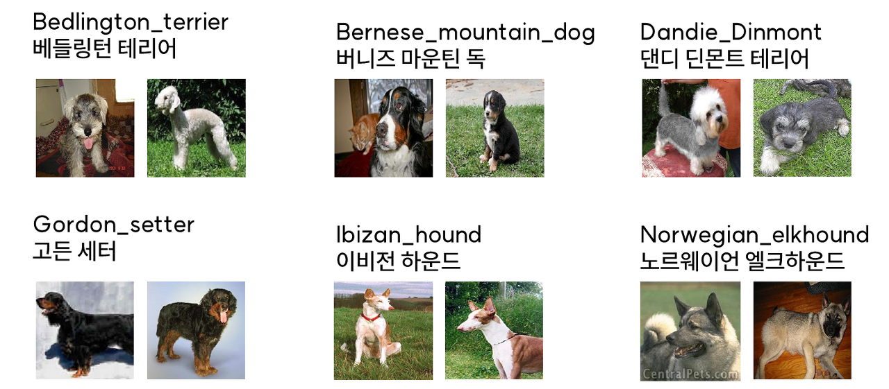
- 이 데이터셋에는 6종류의 개 이미지가 있음
- 파일의 형식은 JPEG이고 이름은 사진 속 개의 품종을 알려줌
- 사진은 견종에 따라 다른 폴더에 저장되어있음
견종 이미지 분류
학습순서에 대한 간단한 설명과 방법
- 다양한 견종 이미지를 훈련시켜 견종을 분류했음
- 처음에는 CNN 구조를 이용해 결과를 보고, pre-trained EfficientNetB5 모델을 사용하여 비교해보기로 함
- 이전 글에선 CNN 구조를 이용해 결과를 확인했고 이번엔 사전 훈련된 모델을 사용함
- 작성된 코드를 참고하여 코드를 분석 및 학습을 진행함
코드 분석 및 학습 내용
사전 훈련된 EfficientNetB5 모델 사용
- EfficientNetB5 모델을 사용했다는 것 외에 이전 코드와 크게 차이는 없음
- 하지만 성능면에서는 높은 점수를 받음
- 이미지를 0에서 1 사이 값으로 정규화 하는 과정을 거치면 성능히 급격히 낮아짐 (추후 공부하여 추가 예정)
Import Necessary Libraries
- 데이터 처리, 머신 러닝 모델 구축, 성능 평가, 시각화 등 다양한 작업을 수행함
- os : 운영 체제 관련 기능을 제공하는 Python 라이브러리
- glob : 파일 경로를 패턴으로 검색할 때 사용되는 라이브러리
- random : 난수 생성 및 관련 기능을 제공하는 라이브러리
- numpy : 수학 및 과학 계산을 위한 Python 라이브러리
- pandas : 데이터 조작 및 분석을 위한 Python 라이브러리
- PIL : 이미지 처리와 조작을 위한 라이브러리
- itertools : 반복 가능한 데이터를 조작하는 데 사용되는 라이브러리
- sklearn : 머신 러닝 및 데이터 분석을 위한 Python 라이브러리
- seaborn : 데이터 시각화를 위한 Python 라이브러리
- matplotlib.pyplot.as plt : 데이터 시각화 및 그래프 생성에 사용되는 Matplotlib의 서브모듈
- tensorflow : 딥러닝 및 기계 학습 라이브러리
- tf.config.optimizer.set_experimental_options : TensorFlow의 실험적인 옵티마이저 옵션을 설정하는 데 사용
import os
import glob
import random

import numpy as np
import pandas as pd
from PIL import Image
from itertools import cycle

from sklearn.model_selection import train_test_split
from sklearn.metrics import confusion_matrix
from sklearn.metrics import accuracy_score
from sklearn.metrics import precision_score
from sklearn.metrics import recall_score
from sklearn.metrics import f1_score
from sklearn.metrics import classification_report
from sklearn.metrics import roc_curve
from sklearn.metrics import auc

from sklearn.preprocessing import LabelEncoder
from sklearn.preprocessing import label_binarize
from keras.utils import to_categorical

import seaborn as sns
import matplotlib.pyplot as plt

import tensorflow as tf
from tensorflow.keras import regularizers
from tensorflow.keras.preprocessing.image import load_img, img_to_array, ImageDataGenerator
from tensorflow.keras.applications import EfficientNetB5
from tensorflow.keras.layers import Dense, GlobalAveragePooling2D
from tensorflow.keras.models import Model
from keras.models import Sequential
from keras.layers import Conv2D, MaxPooling2D, Flatten, Dense, Dropout, BatchNormalization
from keras.optimizers import Adam, Adamax
from keras.callbacks import EarlyStopping, LearningRateScheduler


tf.config.optimizer.set_experimental_options({'layout_optimizer': False})

print ('modules loaded')
modules loaded
# tensorflow device 확인
from tensorflow.python.client import device_lib
device_lib.list_local_devices()
[name: "/device:CPU:0"
 device_type: "CPU"
 memory_limit: 268435456
 locality {
 }
 incarnation: 64955830953055254
 xla_global_id: -1,
 name: "/device:GPU:0"
 device_type: "GPU"
 memory_limit: 5967581184
 locality {
   bus_id: 1
   links {
   }
 }
 incarnation: 2828612098316059951
 physical_device_desc: "device: 0, name: NVIDIA GeForce RTX 2070, pci bus id: 0000:65:00.0, compute capability: 7.5"
 xla_global_id: 416903419]
Load and Preview the Data
- 순서대로 견종 디렉터리에 접근 후 이미지를 읽을 수 있는지 확인하고 이미지와 레이블을 리스트에 추가함
path = './data'
breeds = os.listdir(path)

print('before sort')
print(breeds)

breeds.sort()# Sorting is needed due to correction of labeling
print()

print('after sorted')
print(breeds)
before sort
['Bedlington_terrier', 'Bernese_mountain_dog', 'Dandie_Dinmont', 'Gordon_setter', 'Ibizan_hound', 'Norwegian_elkhound']

after sorted
['Bedlington_terrier', 'Bernese_mountain_dog', 'Dandie_Dinmont', 'Gordon_setter', 'Ibizan_hound', 'Norwegian_elkhound']
images, labels = [], []

for breed in breeds:
    breed_path = os.path.join(path, breed)
    for img_path in glob.glob(breed_path + '/*.jpg'):
        # 이미지를 열어서 읽을 수 있는지 확인함
        with open(img_path, 'rb') as f:
            Image.open(f)
        # 이미지를 읽을 수 있다면, 이미지와 레이블을 리스트에 추가함
        images.append(img_path)
        labels.append(breed)

print('Checking data labeling')
for i in range(0, 600, 100):
    print(images[i] + '        ' + labels[i])
Checking data labeling
./data\Bedlington_terrier\Bedlington_terrier_1.jpg        Bedlington_terrier
./data\Bedlington_terrier\Bedlington_terrier_67.jpg        Bedlington_terrier
./data\Bernese_mountain_dog\Bernese_mountain_dog_39.jpg        Bernese_mountain_dog
./data\Dandie_Dinmont\Dandie_Dinmont_25.jpg        Dandie_Dinmont
./data\Gordon_setter\Gordon_setter_115.jpg        Gordon_setter
./data\Ibizan_hound\Ibizan_hound_100.jpg        Ibizan_hound
Data Preprocessing
- 이미지 크기 조정, 정규화, 학습 및 테스트 세트 분할, 데이터 증강 과정을 거침
input_size = 224


def preprocess_image(image_path, target_size=(input_size, input_size)):

    img = Image.open(image_path)

    # 이미지 크기 조정 및 배열로 전환
    img_resized = img.resize(target_size) # 224 * 224
    img_array = img_to_array(img_resized)
    # img_array = img_array / 255.0 # 이미지를 0에서 1 사이 값으로 정규화 함

    return img_array

# 모든 이미지에 대해 전처리를 수행하고 결과를 리스트에 저장
img_array = [preprocess_image(img_path) for img_path in images]
# 이미지 배열 및 레이블을 시각화하는 함수 정의
def show_images(image_array, labels, encoded_labels=None,images_per_row=5):

    # 랜덤하게 이미지 배열과 레이블을 선택함
    selected_indices = random.sample(range(len(image_array)), images_per_row)
    selected_array = [image_array[i] for i in selected_indices]
    selected_labels = [labels[i] for i in selected_indices]
    try:
        selected_encoded_labels = [encoded_labels[i] for i in selected_indices]
    except:
        selected_encoded_labels = [""] * images_per_row

    # 행의 수 계산
    num_rows = 1 # 한 행에 이미지를 모두 표시하도록 함

    # 이미지를 표시하기 위해 그림과 축을 생성함.
    fig, axes = plt.subplots(num_rows, images_per_row, figsize=(20, 3 * num_rows)) # subplots()  여러개의 그래프를 바둑판식으로 배열하여 나타냄

    # 이미지와 레이블을 반복하면서 시각화함
    for idx, (selected_array, selected_label, selected_encoded_label) in enumerate(zip(selected_array, selected_labels, selected_encoded_labels)):
        # 이미지 픽셀 값을 0-1 범위에서 0-255 범위로 다시 조정함.
        selected_array = selected_array.astype('uint8')
        # selected_array = (selected_array * 255).astype('uint8')

        # NumPy 배열에서 PIL 이미지를 생성함
        img = Image.fromarray(selected_array)
        # 이미지와 해당 레이블을 표시함
        ax = axes[idx]
        ax.imshow(img)
        ax.set_title(f"label: {selected_label}\n encoded_label:{selected_encoded_label}")
        ax.axis('on')  # 축을 비활성화하여 이미지만 표시함

    plt.show()
# 데이터를 전처리하고 변환함.
def data_preprocessing(images, labels):
    # 이미지를 전처리하여 X에 저장
    X = [preprocess_image(img_path) for img_path in images]

    # 레이블을 숫자로 인코딩 (LabelEncoder를 사용해 각 품종을 숫자로 변환)
    y = LabelEncoder().fit_transform(labels)
    # 원-핫 인코딩 (레이블을 다중 클래스 형식으로 변환)
    y = to_categorical(y, num_classes=len(breeds)) # breeds : 품종의 종류

    # 리스트를 넘파이 배열로 변환
    X = np.array(X)
    y = np.array(y)

    return X, y

# 데이터 전처리 함수를 사용하여 이미지와 레이블을 변환
X, y = data_preprocessing(images, labels)
# 데이터를 학습 세트와 검증 세트로 분할함
X_train, X_test, y_train, y_test = train_test_split(X, y, test_size=0.2, random_state=98, stratify=y)
# X : 이미지 데이터
# y : 레이블
# test_size : 검증 세트의 크기를 나타냄
# random_state : 무작위 분할을 제어하는 데 사용되는 시드
# stratify : 레이블 y를 기반으로 계층화 샘플링을 수행함

# 분할된 데이터의 크기를 출력함
print(f"X_train {len(X_train)}")
print(f"X_test, {len(X_test)}")
print(f"y_train, {len(y_train)}")
print(f"y_test {len(y_test)}")
X_train 601
X_test, 151
y_train, 601
y_test 151
# 원-핫 인코딩된 레이블을 디코딩하여 원래의 레이블로 변환하는 함수 정의
def decode_one_hot(one_hot_encoded, labels):
    # 각 행에서 '1'의 위치(인덱스)를 찾기 위해 numpy의 argmax 함수를 사용함
    # axis=1을 지정하여 각 행에서 최대값을 찾음
    indices = np.argmax(one_hot_encoded, axis=1)

    # 인덱스를 사용하여 각 행의 원래 레이블을 찾아서 리스트로 저장함
    decoded_labels = [labels[index] for index in indices]
    return decoded_labels
print('Example of label and one_hot_encoded label')
train_labels = decode_one_hot(y_train, breeds)
show_images(image_array= X_train, labels=train_labels, encoded_labels=y_train)
Example of label and one_hot_encoded label

# 데이터 증강 함수 정의
def data_augmentation(X, y, multiply=2):

    # 데이터 증강을 위한 ImageDataGenerator 객체를 생성함
    datagen = ImageDataGenerator(
        rotation_range=40,
        width_shift_range=0.2,
        height_shift_range=0.2,
        shear_range=0.2,
        zoom_range=0.3,
        horizontal_flip=True,
        vertical_flip=True,
        fill_mode='nearest'
    )

    # 증강된 데이터를 저장할 빈 배열을 생성함
    X_result = np.zeros((len(X) * multiply, *X.shape[1:]), dtype=X.dtype)
    y_result = np.zeros((len(y) * multiply, *y.shape[1:]), dtype=y.dtype)

    # ImageDataGenerator에 원본 데이터를 적용함
    datagen.fit(X)

    i = 0
    for X_batch, y_batch in datagen.flow(X, y, batch_size=len(X), shuffle=False):
        # 증강된 데이터를 결과 배열에 저장함
        X_result[i*len(X):(i+1)*len(X)] = X_batch
        y_result[i*len(y):(i+1)*len(y)] = y_batch
        i += 1
        if i >= multiply:
            break

    return X_result, y_result

# 데이터 증강 함수를 사용해 학습 데이터를 증강함
X_train_augmented, y_train_augmented = data_augmentation(X_train, y_train, multiply=4)
print(f'X_train {X_train.shape}')
print(f'y_train {y_train.shape}')

print()
print('After performed a data augmentation')
print()

print(f'X_train_augmented {X_train_augmented.shape}')
print(f'y_train_augmented {y_train_augmented.shape}')
X_train (601, 224, 224, 3)
y_train (601, 6)

After performed a data augmentation

X_train_augmented (2404, 224, 224, 3)
y_train_augmented (2404, 6)
print('Example of label and one_hot_encoded label of augmentated images')
train_labels = decode_one_hot(y_train_augmented, breeds)
show_images(image_array= X_train_augmented, labels=train_labels, encoded_labels=y_train_augmented)
Example of label and one_hot_encoded label of augmentated images

Model Training
- 모델을 생성하고 모델을 훈련하여 시각화함
tf.__version__
'2.10.0'
def create_model(learning_rate=0.0001):
    # Load the pre-trained EfficientNetB5 model
    base_model = EfficientNetB5(weights='imagenet', include_top=False, input_shape=(input_size, input_size, 3), pooling= 'max')
    base_model.trainable = False

    # Sequential 모델을 생성함
    model = Sequential([
        base_model,
        BatchNormalization(axis= -1, momentum= 0.99, epsilon= 0.001),
        Dense(128, kernel_regularizer= regularizers.l2(l= 0.016), activity_regularizer= regularizers.l1(0.006),
                bias_regularizer= regularizers.l1(0.006), activation= 'relu'),
        Dropout(rate= 0.45, seed= 123), # 드롭아웃 레이어 : 드롭아웃 비율 (과적합 방지)

        # 출력 레이어 : 견종 수에 해당하는 뉴런 수와 softmax 활성화 함수
        Dense(len(breeds), activation='softmax')
    ])

    model.summary() # 모델 요약 정보 출력

    # 모델 컴파일 : Adamax 옵티마이저
    model.compile(optimizer=Adam(learning_rate=learning_rate), loss='categorical_crossentropy', metrics=['accuracy'])
    return model
# Fit the model
def fit_model(model,X_train, y_train, epochs=50, batch_size=64):

    history = model.fit(
        X_train,   # 입력 데이터
        y_train,   # 출력 데이터 (레이블)
        validation_split=0.2, # 검증 데이터 비율
        epochs=epochs, # 전체 훈련 반복 횟수
        batch_size=batch_size, # 배치 크기
        verbose=0) # 훈련 과정 출력 여부 (0: 출력하지 않음)

    return history # 훈련 과정의 히스토리 객체
# Visualize Training Progress
def plot(history):
    # 그래프의 크기를 설정하고 1*2 그래프를 생성함
    fig, axes = plt.subplots(1, 2, figsize=(14, 5))  # 1 row, 2 columns

    # 정확도 그래프 그림
    axes[0].plot(history.history['accuracy'], label='accuracy')
    axes[0].plot(history.history['val_accuracy'], label='val_accuracy')
    axes[0].set_xlabel('Epoch')
    axes[0].set_ylabel('Accuracy')
    axes[0].legend()
    axes[0].set_title('Model Accuracy')

    # 손실 그래프 그림
    axes[1].plot(history.history['loss'], label='loss')
    axes[1].plot(history.history['val_loss'], label='val_loss')
    axes[1].set_xlabel('Epoch')
    axes[1].set_ylabel('Loss')
    axes[1].legend()
    axes[1].set_title('Model Loss')

    # 그래프를 조밀하게 배치하고 출력함
    plt.tight_layout()
    plt.show()
batch_size = 64

model = create_model(learning_rate=0.0001)
history = fit_model(model,X_train_augmented, y_train_augmented, epochs= 30, batch_size=16)
plot(history)
Model: "sequential_7"
_________________________________________________________________
 Layer (type)                Output Shape              Param #
=================================================================
 efficientnetb5 (Functional)  (None, 2048)             28513527

 batch_normalization_7 (Batc  (None, 2048)             8192
 hNormalization)

 dense_14 (Dense)            (None, 128)               262272

 dropout_7 (Dropout)         (None, 128)               0

 dense_15 (Dense)            (None, 6)                 774

=================================================================
Total params: 28,784,765
Trainable params: 267,142
Non-trainable params: 28,517,623
_________________________________________________________________

Model Evaluation
- 모델을 사용해 이미지에 대한 견종 예측을 수행한 후 분류 성능을 측정하고 ROC 곡선을 시각화함
# 모델을 사용해 이미지 배열에 대한 견종 예측을 수행하는 함수
def predict_breeds( model, img_array):
    #이미지 배열을 Numpy 배열로 변환함
    img_array = np.array(img_array)

    # 이미지 배열이 3차원이라면 4차원으로 확장함
    if len(img_array.shape) == 3:
        img_array = np.expand_dims(img_array, axis=0)

    # 모델을 사용해 여러 이미지에 대한 예측을 수행함
    predictions = model.predict(img_array)

    # 가장 높은 확률을 가진 클래스의 인덱스를 찾음
    predicted_indices = np.argmax(predictions, axis=1)

    # 예측된 인덱스를 해당하는 견종 레이블로 매핑함
    predicted_breeds = [breeds[index] for index in predicted_indices]

    return predicted_breeds
# 예측 수행 후 예측 결과 시각화 함수
def show_images_with_predicted_results(model, image_array, labels, images_per_row=5):

    # 모델로 이미지 예측 수행
    predicted_labels = predict_breeds(model, image_array)


    # 이미지 배열 중 일부 무작위로 선택함
    selected_indices = random.sample(range(len(image_array)), images_per_row)
    selected_arrays = [image_array[i] for i in selected_indices]
    selected_labels = [labels[i] for i in selected_indices]
    selected_preds = [predicted_labels[i] for i in selected_indices]

    # 행의 수 결정
    num_rows = 1

    # 이미지와 예측 결과를 표시할 그림과 축을 생성함
    fig, axes = plt.subplots(num_rows, images_per_row, figsize=(20, 3 * num_rows))

    # 이미지와 레이블을 반복하며 표시함
    for idx, (img_array, true_label, pred_label) in enumerate(zip(selected_arrays, selected_labels, selected_preds)):
        # 픽셀 값을 0-1 범위내에서 0-255 범위로 재조정함
        #img_array = (img_array * 255).astype('uint8')
        img_array = img_array.astype('uint8')

        # Numpy 배열에서 PIL 이미지를 생성함
        img = Image.fromarray(img_array)

        # 이미지와 해당 레이블을 표시함
        ax = axes[idx]
        ax.imshow(img)
        ax.set_title(f"True: {true_label} \n Pred: {pred_label}")
        ax.axis('on')  # 축을 끔

    # 이미지와 예측 결과 표시함
    plt.show()
print('Example of predicted images')
decoded_y_test = decode_one_hot(y_test, breeds)
show_images_with_predicted_results(model, X_test, decoded_y_test)
Example of predicted images
5/5 [==============================] - 50s 6s/step

# 모델을 사용해 예측하고 혼동 행렬 시각화하는 함수
def predict_and_plot_confusion_matrix(model, X, y_true):
    # 모델을 사용해 클래스를 예측함
    y_pred = model.predict(X)
    predicted_classes = np.argmax(y_pred, axis=1)

    # 원-핫 인코딩된 실제 레이블을 디코딩함
    true_classes = np.argmax(y_true, axis=1)


    # 혼동 행렬을 계산함
    cm = confusion_matrix(true_classes, predicted_classes)


    # 시각화를 위한 히트맵을 생성함
    plt.figure(figsize=(8, 6))
    sns.heatmap(cm, annot=True, fmt="d", cmap="Blues", xticklabels=breeds, yticklabels=breeds)
    plt.xlabel('Predicted Labels')
    plt.ylabel('True Labels')
    plt.title('Confusion Matrix of a Test Set')
    plt.show()

# 테스트 데이터에 대한 혼동 행렬을 출력함
predict_and_plot_confusion_matrix(model, X = X_test, y_true = y_test)
5/5 [==============================] - 15s 4s/step

y_test_pred_probs = model.predict(X_test)
y_test_pred = np.argmax(y_test_pred_probs, axis=1)
y_test_true = np.argmax(y_test, axis=1)


accuracy = accuracy_score(y_test_true, y_test_pred)
precision = precision_score(y_test_true, y_test_pred, average='weighted')
recall = recall_score(y_test_true, y_test_pred, average='weighted')
f1 = f1_score(y_test_true, y_test_pred, average='weighted')

print(f"Accuracy: {accuracy:.4f}")
print(f"Precision: {precision:.4f}")
print(f"Recall: {recall:.4f}")
print(f"F1 Score: {f1:.4f}")
5/5 [==============================] - 15s 4s/step
Accuracy: 0.9934
Precision: 0.9937
Recall: 0.9934
F1 Score: 0.9934
report = classification_report(y_test_true, y_test_pred, target_names=breeds)
print(report)
                      precision    recall  f1-score   support

  Bedlington_terrier       1.00      0.96      0.98        28
Bernese_mountain_dog       1.00      1.00      1.00        26
      Dandie_Dinmont       0.96      1.00      0.98        23
       Gordon_setter       1.00      1.00      1.00        23
        Ibizan_hound       1.00      1.00      1.00        25
  Norwegian_elkhound       1.00      1.00      1.00        26

            accuracy                           0.99       151
           macro avg       0.99      0.99      0.99       151
        weighted avg       0.99      0.99      0.99       151
# Binarize the labels
y_test_bin = label_binarize(y_test, classes=breeds)  # 각 클래스를 이진화함

# Compute ROC curve and ROC area for each class
fpr = dict()  # False Positive Rate를 저장할 딕셔너리
tpr = dict()  # True Positive Rate를 저장할 딕셔너리
roc_auc = dict()  # ROC 곡선 아래 면적을 저장할 딕셔너리
n_classes = y_test_bin.shape[1]  # 클래스의 개수
y_score = model.predict(X_test)  # 모델에서 예측한 확률 점수를 얻음

# 각 클래스에 대한 ROC 곡선과 면적을 계산함
for i in range(n_classes):
    fpr[i], tpr[i], _ = roc_curve(y_test_bin[:, i], y_score[:, i])  # 클래스 별 ROC 곡선을 계산함
    roc_auc[i] = auc(fpr[i], tpr[i])  # 클래스 별 ROC 곡선 아래 면적을 계산함

# Compute micro-average ROC curve and ROC area
fpr["micro"], tpr["micro"], _ = roc_curve(y_test_bin.ravel(), y_score.ravel())  # Micro-average ROC 곡선을 계산함
roc_auc["micro"] = auc(fpr["micro"], tpr["micro"])  # Micro-average ROC 곡선 아래 면적을 계산함

# Plot ROC curve for micro-average
plt.figure(figsize=(8, 6))
plt.plot(fpr["micro"], tpr["micro"], color='b', label=f'Micro-average ROC curve (area = {roc_auc["micro"]:0.2f})')

plt.plot([0, 1], [0, 1], 'k--')  # 대각선 직선을 그림
plt.xlim([0.0, 1.0])  # X 축 범위 설정
plt.ylim([0.0, 1.05])  # Y 축 범위 설정
plt.xlabel('False Positive Rate')  # X 축 레이블 설정
plt.ylabel('True Positive Rate')  # Y 축 레이블 설정
plt.title('ROC Curve with Micro-Average')  # 그래프 제목 설정
plt.legend(loc="lower right")  # 범례 위치 설정
plt.show()  # 그래프를 표시함
5/5 [==============================] - 15s 4s/step

'개인 공부 > 인공지능' 카테고리의 다른 글
| [딥러닝] 대규모 언어 모델(LLM) (0) | 2025.08.26 |
|---|---|
| [딥러닝] 순환 신경망(Recurrent Neural Network, RNN) (0) | 2024.03.27 |
| [kaggle/Flask] 견종 분류 모델 웹에 구현하기 (1) | 2023.10.04 |
| [kaggle/TensorFlow] 견종 이미지 분류 모델 구현 - 1 (0) | 2023.09.26 |
| [GPU설정] CUDA 환경 구성 (Tensorflow, PyTorch) (1) | 2023.09.25 |


